Scanpy PBMC quickstart#
Audience:
Single-cell researchers and analysts who already use Scanpy and want the shortest baseline path from
AnnDatato a learned embedding.
Prerequisites:
Install
scdlkit[tutorials].Familiarity with
AnnData, neighbors, and UMAP in Scanpy.
Learning goals:
Load PBMC data with Scanpy.
Train a VAE baseline with
TaskRunner.Store latent embeddings in
adata.obsm.Continue with Scanpy neighbors and UMAP on the learned representation.
Out of scope:
raw-count QC and preprocessing
marker-gene interpretation
gene-level reconstruction inspection
Why this notebook starts from processed PBMC:
scDLKit is focusing here on the model layer, not reproducing the full raw preprocessing tutorial that Scanpy already teaches well.
The raw-count preprocessing path stays in the official Scanpy tutorials; this notebook starts at the point where model training begins.
Install:
python -m pip install "scdlkit[tutorials]"
Links:
Repository: uddamvathanak/scDLKit
Related APIs:
TaskRunner: stable beginner workflowprepare_data(...): lower-level preprocessing and split control
Next steps:
Tutorial:
downstream_scanpy_after_scdlkit.ipynbAPI:
docs/api/taskrunner.md
Published tutorial status
This page is a static notebook copy published for documentation review. It is meant to show the exact workflow and outputs from the last recorded run.
Last run date (UTC):
2026-03-27 09:22 UTCPublication mode:
static executed tutorialExecution profile:
publishedArtifact check in this sync:
passedSource notebook:
examples/train_vae_pbmc.ipynb
Outline#
Load PBMC data with Scanpy.
Inspect the dataset and confirm the label field.
Detect the runtime device.
Choose the notebook profile.
Train a VAE with
device="auto".Evaluate metrics and save artifacts.
Push the latent embedding into
adata.obsm.Run Scanpy neighbors and UMAP on the latent space.
from __future__ import annotations

from pathlib import Path

import scanpy as sc
import torch
from IPython.display import display

from scdlkit import TaskRunner

sc.set_figure_params(dpi=100, dpi_save=180, frameon=False, fontsize=12)

DATA_PATH = Path("examples/data/pbmc3k_processed.h5ad")
OUTPUT_DIR = Path("artifacts/pbmc_vae_quickstart")
OUTPUT_DIR.mkdir(parents=True, exist_ok=True)

device_name = "cuda" if torch.cuda.is_available() else "cpu"
print(f"Using device: {device_name}")
Using device: cpu
TUTORIAL_PROFILE = "quickstart"  # change to "full" for a longer run

PROFILE = {
    "quickstart": {"epochs": 20, "batch_size": 128, "kl_weight": 1e-3},
    "full": {"epochs": 50, "batch_size": 128, "kl_weight": 1e-3},
}[TUTORIAL_PROFILE]

print(f"Tutorial profile: {TUTORIAL_PROFILE}")
print(PROFILE)
Tutorial profile: quickstart
{'epochs': 20, 'batch_size': 128, 'kl_weight': 0.001}
Load PBMC data#
The tutorial prefers the repository copy of pbmc3k_processed.h5ad when available, then falls back to scanpy.datasets.pbmc3k_processed().
adata = sc.read_h5ad(DATA_PATH) if DATA_PATH.exists() else sc.datasets.pbmc3k_processed()
print(adata)
print(f"Shape: {adata.shape}")
print("obs columns:", list(adata.obs.columns))
print("Label field used for evaluation:", "louvain")
AnnData object with n_obs × n_vars = 2638 × 1838
    obs: 'n_genes', 'percent_mito', 'n_counts', 'louvain'
    var: 'n_cells'
    uns: 'draw_graph', 'louvain', 'louvain_colors', 'neighbors', 'pca', 'rank_genes_groups'
    obsm: 'X_pca', 'X_tsne', 'X_umap', 'X_draw_graph_fr'
    varm: 'PCs'
    obsp: 'distances', 'connectivities'
Shape: (2638, 1838)
obs columns: ['n_genes', 'percent_mito', 'n_counts', 'louvain']
Label field used for evaluation: louvain
Train the VAE baseline#
This is the main scDLKit step. The code is the same on CPU and GPU because the runner uses device="auto".
For this PBMC quickstart, the VAE uses a light KL term so PBMC populations stay visibly separated in the latent space. A healthy quickstart result should show broad islands for major PBMC groups rather than a single mixed circular cloud.
Use the default quickstart profile for a CPU-friendly docs run. Switch to full when you want a longer fit with stronger qualitative separation before interpreting the embedding.
runner = TaskRunner(
    model="vae",
    task="representation",
    epochs=PROFILE["epochs"],
    batch_size=PROFILE["batch_size"],
    label_key="louvain",
    device="auto",
    model_kwargs={"kl_weight": PROFILE["kl_weight"]},
    output_dir=str(OUTPUT_DIR),
)
runner.fit(adata)
metrics = runner.evaluate()
metrics
{'mse': 0.8214080929756165,
 'mae': 0.40160080790519714,
 'pearson': 0.22945579886436462,
 'spearman': 0.12458946432617383,
 'silhouette': 0.17217771708965302,
 'knn_label_consistency': 0.8914141414141414,
 'ari': 0.5968597655832685,
 'nmi': 0.762229436266658}
What to inspect#
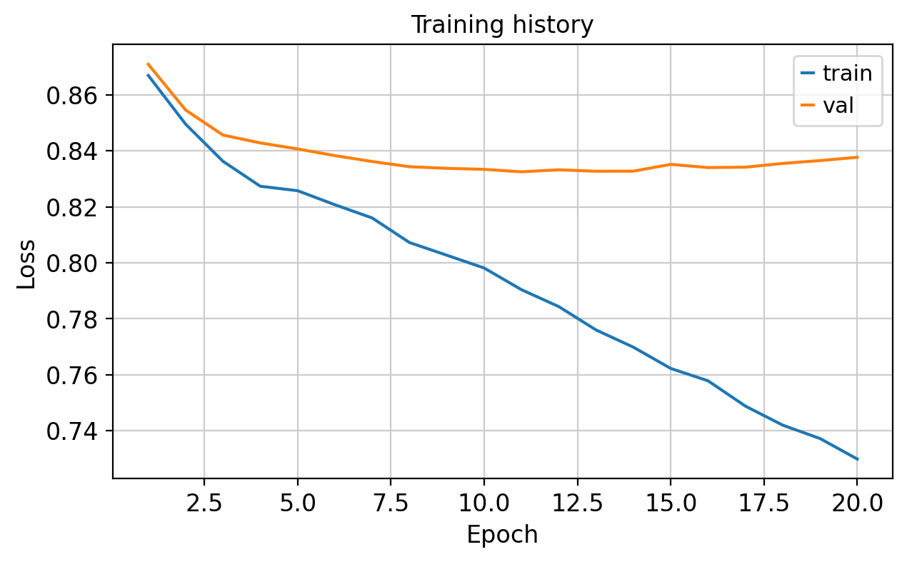
Before moving on, check three things:
The training curve should fall without obvious instability.
The latent UMAP should separate broad PBMC families rather than collapsing into a single mixed blob.
This notebook is only the embedding step. Marker-gene interpretation and reconstruction inspection live in separate tutorials.
The notebook writes a Markdown report and a training-loss plot to artifacts/pbmc_vae_quickstart/.
runner.save_report(OUTPUT_DIR / "report.md")
loss_fig, _ = runner.plot_losses()
loss_fig.savefig(OUTPUT_DIR / "loss_curve.png", dpi=150, bbox_inches="tight")
display(loss_fig)
Push the latent space back into Scanpy#
scDLKit stays model-focused. Once the latent representation is available, continue the downstream neighborhood and visualization workflow with Scanpy.
A healthy result should show broad louvain groups separating into distinct islands rather than a single mixed circular cloud.
adata.obsm["X_scdlkit_vae"] = runner.encode(adata)
sc.pp.neighbors(adata, use_rep="X_scdlkit_vae")
sc.tl.umap(adata, random_state=42)
umap_fig = sc.pl.umap(
    adata,
    color="louvain",
    legend_loc="on data",
    legend_fontsize=10,
    legend_fontoutline=2,
    title="",
    return_fig=True,
    frameon=False,
)
umap_fig.savefig(OUTPUT_DIR / "latent_umap.png", dpi=150, bbox_inches="tight")
display(umap_fig)
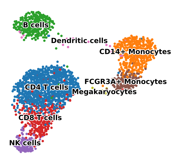
Expected outputs#
After running this notebook you should have:
metrics from
runner.evaluate()artifacts/pbmc_vae_quickstart/report.mdartifacts/pbmc_vae_quickstart/report.csvartifacts/pbmc_vae_quickstart/loss_curve.pngartifacts/pbmc_vae_quickstart/latent_umap.pnga latent UMAP with broad separation between PBMC populations such as T cells, B cells, monocytes, and NK cells
Recommended next steps:
re-run the first config cell with
TUTORIAL_PROFILE = "full"when you want a stronger qualitative resultopen the downstream Scanpy tutorial for clustering, markers, and broad annotation after the embedding step
open the PBMC model-comparison tutorial to compare
PCA,autoencoder,vae, andtransformer_aeon the same datasetopen the reconstruction sanity-check tutorial if you want to inspect predicted or reconstructed gene-expression values
output_paths = {
    "report_md": str(OUTPUT_DIR / "report.md"),
    "report_csv": str(OUTPUT_DIR / "report.csv"),
    "loss_curve_png": str(OUTPUT_DIR / "loss_curve.png"),
    "latent_umap_png": str(OUTPUT_DIR / "latent_umap.png"),
}
output_paths
{'report_md': 'artifacts/pbmc_vae_quickstart/report.md',
 'report_csv': 'artifacts/pbmc_vae_quickstart/report.csv',
 'loss_curve_png': 'artifacts/pbmc_vae_quickstart/loss_curve.png',
 'latent_umap_png': 'artifacts/pbmc_vae_quickstart/latent_umap.png'}