Downstream Scanpy after scDLKit#
Audience:
Researchers and analysts who already trained a baseline model and now want the missing interpretation layer after the embedding step.
Prerequisites:
Install
scdlkit[tutorials].Know the main PBMC quickstart notebook first.
Be comfortable with
AnnData,adata.obsm, neighbors, and UMAP in Scanpy.
Learning goals:
train a scDLKit baseline and reuse the embedding in Scanpy
cluster the latent embedding with Leiden
rank marker genes for the latent-space clusters
visualize broad PBMC marker patterns with a dotplot
make a careful coarse annotation pass and compare back to the reference PBMC labels
Out of scope:
raw-count QC and preprocessing
marker validation beyond broad tutorial-level checks
publication-grade biological interpretation
This notebook starts from pbmc3k_processed() on purpose. scDLKit owns the model-training layer here; the raw preprocessing path remains covered by the official Scanpy tutorials.
Published tutorial status
This page is a static notebook copy published for documentation review. It is meant to show the exact workflow and outputs from the last recorded run.
Last run date (UTC):
2026-03-27 09:23 UTCPublication mode:
static executed tutorialExecution profile:
publishedArtifact check in this sync:
passedSource notebook:
examples/downstream_scanpy_after_scdlkit.ipynb
Outline#
Load processed PBMC data.
Train a VAE baseline and produce a latent embedding.
Build the neighbor graph and UMAP from
adata.obsm.Run Leiden clustering on the scDLKit embedding.
Rank marker genes and visualize a broad marker panel.
Compare the new latent-space clusters back to the reference PBMC labels.
Save a short downstream report and output artifact paths.
from __future__ import annotations

from pathlib import Path

import numpy as np
import pandas as pd
import scanpy as sc
import torch
from IPython.display import display
from matplotlib import pyplot as plt
from sklearn.metrics import adjusted_rand_score
from sklearn.model_selection import train_test_split

from scdlkit import TaskRunner
from scdlkit.evaluation import save_markdown_report, save_metrics_table

sc.set_figure_params(dpi=100, dpi_save=180, frameon=False, fontsize=12)

OUTPUT_DIR = Path("artifacts/downstream_scanpy_after_scdlkit")
OUTPUT_DIR.mkdir(parents=True, exist_ok=True)

TUTORIAL_PROFILE = "quickstart"  # change to "full" for the full dataset
PROFILE = {
    "quickstart": {"max_cells": 1500, "epochs": 15, "batch_size": 128},
    "full": {"max_cells": None, "epochs": 35, "batch_size": 128},
}[TUTORIAL_PROFILE]

print(f"Using device: {'cuda' if torch.cuda.is_available() else 'cpu'}")
print(f"Tutorial profile: {TUTORIAL_PROFILE}")
print(PROFILE)
Using device: cpu
Tutorial profile: quickstart
{'max_cells': 1500, 'epochs': 15, 'batch_size': 128}
Load PBMC data#
The quickstart profile uses a deterministic stratified subset so the docs build stays affordable. The full profile keeps all processed PBMC cells.
def stratified_subset(adata, label_key: str, max_cells: int | None, seed: int = 42):
    if max_cells is None or adata.n_obs <= max_cells:
        return adata.copy()
    indices = np.arange(adata.n_obs)
    labels = adata.obs[label_key].astype(str).to_numpy()
    keep_indices, _ = train_test_split(
        indices,
        train_size=max_cells,
        random_state=seed,
        stratify=labels,
    )
    return adata[np.sort(keep_indices)].copy()

adata = sc.datasets.pbmc3k_processed()
adata = stratified_subset(adata, "louvain", PROFILE["max_cells"])
print(adata)
print("obs columns:", list(adata.obs.columns))
AnnData object with n_obs × n_vars = 1500 × 1838
    obs: 'n_genes', 'percent_mito', 'n_counts', 'louvain'
    var: 'n_cells'
    uns: 'draw_graph', 'louvain', 'louvain_colors', 'neighbors', 'pca', 'rank_genes_groups'
    obsm: 'X_pca', 'X_tsne', 'X_umap', 'X_draw_graph_fr'
    varm: 'PCs'
    obsp: 'distances', 'connectivities'
obs columns: ['n_genes', 'percent_mito', 'n_counts', 'louvain']
Train a baseline embedding#
This notebook intentionally reuses the same VAE family as the main quickstart so the downstream differences come from the interpretation layer, not from a different model story.
runner = TaskRunner(
    model="vae",
    task="representation",
    label_key="louvain",
    epochs=PROFILE["epochs"],
    batch_size=PROFILE["batch_size"],
    device="auto",
    model_kwargs={"kl_weight": 1e-3},
    output_dir=str(OUTPUT_DIR / "runner"),
)
runner.fit(adata)
train_metrics = runner.evaluate()
latent = runner.encode(adata)
adata.obsm["X_scdlkit_vae"] = latent
train_metrics
{'mse': 0.8118735551834106,
 'mae': 0.4016185402870178,
 'pearson': 0.2227245718240738,
 'spearman': 0.11818246858977441,
 'silhouette': 0.16567520797252655,
 'knn_label_consistency': 0.8755555555555555,
 'ari': 0.5356517210359358,
 'nmi': 0.7194481794557122}
Return to Scanpy for clustering and visualization#
Once the embedding exists in adata.obsm, the rest of the workflow should look familiar to a Scanpy user.
sc.pp.neighbors(adata, use_rep="X_scdlkit_vae")
sc.tl.umap(adata, random_state=42)
sc.tl.leiden(adata, key_added="scdlkit_leiden", flavor="igraph", n_iterations=2)
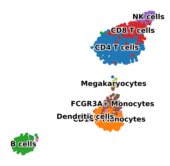
latent_umap = sc.pl.umap(
adata,
color="louvain",
legend_loc="on data",
legend_fontsize=10,
legend_fontoutline=2,
title="",
return_fig=True,
frameon=False,
)
latent_umap.savefig(OUTPUT_DIR / "latent_umap.png", dpi=150, bbox_inches="tight")
display(latent_umap)
plt.close(latent_umap)
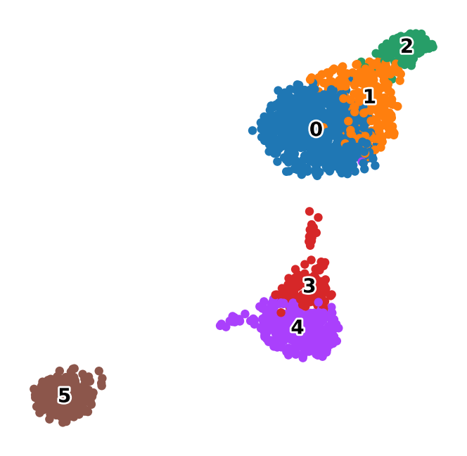
leiden_umap = sc.pl.umap(
adata,
color="scdlkit_leiden",
legend_loc="on data",
legend_fontsize=10,
legend_fontoutline=2,
title="",
return_fig=True,
frameon=False,
)
leiden_umap.savefig(OUTPUT_DIR / "leiden_umap.png", dpi=150, bbox_inches="tight")
display(leiden_umap)
plt.close(leiden_umap)
Rank markers and inspect broad PBMC signatures#
This is the part our older tutorials were missing. The point is not to claim detailed biology, but to show that the scDLKit embedding can be taken through the usual Scanpy interpretation path.
marker_panel = {
    "T_cells": ["IL7R", "LTB"],
    "NK_cells": ["NKG7", "GNLY"],
    "B_cells": ["MS4A1", "CD79A"],
    "Monocytes": ["LYZ", "FCN1"],
    "Dendritic": ["FCER1A", "CST3"],
}
marker_panel = {
    name: [gene for gene in genes if gene in adata.var_names]
    for name, genes in marker_panel.items()
}
marker_panel = {name: genes for name, genes in marker_panel.items() if genes}

sc.tl.rank_genes_groups(adata, groupby="scdlkit_leiden", method="wilcoxon")
rank_df = sc.get.rank_genes_groups_df(adata, group=None)
rank_df.to_csv(OUTPUT_DIR / "rank_genes_groups.csv", index=False)

dotplot = sc.pl.dotplot(
    adata,
    marker_panel,
    groupby="scdlkit_leiden",
    return_fig=True,
    show=False,
)
dotplot.savefig(OUTPUT_DIR / "marker_dotplot.png", dpi=150, bbox_inches="tight")
display(dotplot)
plt.close("all")

rank_df.head()
<scanpy.plotting._dotplot.DotPlot at 0x7f52a4dcbed0>
| group | names | scores | logfoldchanges | pvals | pvals_adj | |
|---|---|---|---|---|---|---|
| 0 | 0 | LDHB | 20.955866 | 1.999101 | 1.658865e-97 | 2.274967e-93 |
| 1 | 0 | CD3D | 20.000904 | 2.308409 | 5.408375e-89 | 3.708522e-85 |
| 2 | 0 | RPS27 | 18.581175 | 0.918824 | 4.564055e-77 | 7.823931e-74 |
| 3 | 0 | RPS27A | 18.571236 | 1.172761 | 5.492466e-77 | 8.369297e-74 |
| 4 | 0 | RPS25 | 18.536173 | 1.006564 | 1.054638e-76 | 1.446331e-73 |
Coarse annotation and comparison back to reference labels#
We keep this annotation deliberately broad. The aim is to sanity-check the latent-space clusters, not to pretend this notebook solves PBMC annotation comprehensively.
def dense_column(adata, gene: str):
    values = adata[:, gene].X
    if hasattr(values, "toarray"):
        values = values.toarray()
    return np.asarray(values).ravel()

score_frame = pd.DataFrame(index=adata.obs_names)
for cell_type, genes in marker_panel.items():
    if not genes:
        continue
    stacked = np.vstack([dense_column(adata, gene) for gene in genes])
    score_frame[cell_type] = stacked.mean(axis=0)

annotation_frame = adata.obs[["louvain", "scdlkit_leiden"]].copy()
if not score_frame.empty:
    annotation_frame = annotation_frame.join(score_frame)
    dominant_scores = annotation_frame.groupby("scdlkit_leiden")[score_frame.columns].mean()
    broad_map = dominant_scores.idxmax(axis=1).to_dict()
    annotation_frame["broad_annotation"] = annotation_frame["scdlkit_leiden"].map(broad_map)
else:
    broad_map = {}
    annotation_frame["broad_annotation"] = "unassigned"

ari_vs_reference = adjusted_rand_score(
    annotation_frame["louvain"].astype(str),
    annotation_frame["scdlkit_leiden"].astype(str),
)
cluster_table = pd.crosstab(annotation_frame["scdlkit_leiden"], annotation_frame["louvain"])
display(cluster_table)
pd.Series(broad_map, name="broad_annotation")
/tmp/ipykernel_2523/3638384049.py:17: FutureWarning: The default of observed=False is deprecated and will be changed to True in a future version of pandas. Pass observed=False to retain current behavior or observed=True to adopt the future default and silence this warning.
  dominant_scores = annotation_frame.groupby("scdlkit_leiden")[score_frame.columns].mean()
| louvain | CD4 T cells | CD14+ Monocytes | B cells | CD8 T cells | NK cells | FCGR3A+ Monocytes | Dendritic cells | Megakaryocytes |
|---|---|---|---|---|---|---|---|---|
| scdlkit_leiden | ||||||||
| 0 | 557 | 0 | 3 | 32 | 0 | 0 | 0 | 0 |
| 1 | 90 | 0 | 0 | 136 | 2 | 1 | 0 | 0 |
| 2 | 0 | 0 | 0 | 12 | 86 | 0 | 0 | 0 |
| 3 | 1 | 25 | 1 | 0 | 0 | 76 | 0 | 9 |
| 4 | 1 | 248 | 0 | 0 | 0 | 8 | 17 | 0 |
| 5 | 1 | 0 | 190 | 0 | 0 | 0 | 4 | 0 |
0      T_cells
1     NK_cells
2     NK_cells
3    Monocytes
4    Monocytes
5      B_cells
Name: broad_annotation, dtype: object
Save a downstream report#
A good tutorial here should leave behind both plots and a short summary so users can tell whether a future feature is behaving reasonably.
summary_metrics = {
    "n_cells": int(adata.n_obs),
    "latent_dim": int(latent.shape[1]),
    "n_leiden_clusters": int(adata.obs["scdlkit_leiden"].nunique()),
    "ari_vs_reference_louvain": float(ari_vs_reference),
}
save_metrics_table(summary_metrics, OUTPUT_DIR / "report.csv")
save_markdown_report(
    summary_metrics,
    path=OUTPUT_DIR / "report.md",
    title="Downstream Scanpy after scDLKit report",
    extra_sections=[
        "## Notes",
        "",
        "- This tutorial starts from processed PBMC data rather than raw counts.",
        "- Use the official Scanpy preprocessing tutorials for QC, filtering, and HVG selection.",
        f"- Broad cluster annotation map: `{broad_map}`",
    ],
)
summary_metrics
{'n_cells': 1500,
 'latent_dim': 32,
 'n_leiden_clusters': 6,
 'ari_vs_reference_louvain': 0.7370774720497316}
Expected outputs#
After running this notebook, check:
artifacts/downstream_scanpy_after_scdlkit/latent_umap.pngartifacts/downstream_scanpy_after_scdlkit/leiden_umap.pngartifacts/downstream_scanpy_after_scdlkit/marker_dotplot.pngartifacts/downstream_scanpy_after_scdlkit/rank_genes_groups.csvartifacts/downstream_scanpy_after_scdlkit/report.md
Interpretation checklist:
The embedding should still preserve broad PBMC structure.
The Leiden clusters should not look obviously mixed or collapsed.
The broad marker panel should line up with the expected PBMC families.
The report is a sanity check, not a claim of complete biological annotation.
Recommended next tutorials:
the PBMC model-comparison notebook for a baseline view against
PCAthe reconstruction sanity-check notebook when you want to inspect predicted or reconstructed gene-expression values
output_paths = {
    "report_md": str(OUTPUT_DIR / "report.md"),
    "report_csv": str(OUTPUT_DIR / "report.csv"),
    "latent_umap_png": str(OUTPUT_DIR / "latent_umap.png"),
    "leiden_umap_png": str(OUTPUT_DIR / "leiden_umap.png"),
    "marker_dotplot_png": str(OUTPUT_DIR / "marker_dotplot.png"),
    "rank_genes_groups_csv": str(OUTPUT_DIR / "rank_genes_groups.csv"),
}
output_paths
{'report_md': 'artifacts/downstream_scanpy_after_scdlkit/report.md',
 'report_csv': 'artifacts/downstream_scanpy_after_scdlkit/report.csv',
 'latent_umap_png': 'artifacts/downstream_scanpy_after_scdlkit/latent_umap.png',
 'leiden_umap_png': 'artifacts/downstream_scanpy_after_scdlkit/leiden_umap.png',
 'marker_dotplot_png': 'artifacts/downstream_scanpy_after_scdlkit/marker_dotplot.png',
 'rank_genes_groups_csv': 'artifacts/downstream_scanpy_after_scdlkit/rank_genes_groups.csv'}