PBMC classification baseline#

Audience:

Researchers who want a simple supervised baseline on a familiar single-cell dataset.

Prerequisites:

Install scdlkit[tutorials].
PBMC data available through Scanpy or the repository cache.

Learning goals:

Train mlp_classifier on PBMC labels.
Inspect accuracy and macro F1.
Plot and save a confusion matrix.
Keep the same notebook path on CPU or GPU with device="auto".

Out of scope:

production-grade annotation
uncertainty calibration
large-scale cell-type labeling workflows

Install:

python -m pip install "scdlkit[tutorials]"

Published tutorial status

This page is a static notebook copy published for documentation review. It is meant to show the exact workflow and outputs from the last recorded run.

Last run date (UTC): 2026-03-27 09:24 UTC
Publication mode: static executed tutorial
Execution profile: published
Artifact check in this sync: passed
Source notebook: examples/classification_demo.ipynb

Outline#

Load PBMC data with Scanpy.
Detect the runtime device.
Choose the notebook profile.
Fit the classification baseline with device="auto".
Evaluate and save a report.
Plot a confusion matrix.

from __future__ import annotations

from pathlib import Path

import scanpy as sc
import torch
from IPython.display import display

from scdlkit import TaskRunner

DATA_PATH = Path("examples/data/pbmc3k_processed.h5ad")
OUTPUT_DIR = Path("artifacts/pbmc_classification")
OUTPUT_DIR.mkdir(parents=True, exist_ok=True)

device_name = "cuda" if torch.cuda.is_available() else "cpu"
print(f"Using device: {device_name}")

Using device: cpu

TUTORIAL_PROFILE = "quickstart"  # change to "full" for a longer run

PROFILE = {
    "quickstart": {"epochs": 15, "batch_size": 128},
    "full": {"epochs": 30, "batch_size": 128},
}[TUTORIAL_PROFILE]

print(f"Tutorial profile: {TUTORIAL_PROFILE}")
print(PROFILE)

Tutorial profile: quickstart
{'epochs': 15, 'batch_size': 128}

adata = sc.read_h5ad(DATA_PATH) if DATA_PATH.exists() else sc.datasets.pbmc3k_processed()
print(adata)
print("Classification target:", "louvain")

AnnData object with n_obs × n_vars = 2638 × 1838
    obs: 'n_genes', 'percent_mito', 'n_counts', 'louvain'
    var: 'n_cells'
    uns: 'draw_graph', 'louvain', 'louvain_colors', 'neighbors', 'pca', 'rank_genes_groups'
    obsm: 'X_pca', 'X_tsne', 'X_umap', 'X_draw_graph_fr'
    varm: 'PCs'
    obsp: 'distances', 'connectivities'
Classification target: louvain

Train the classifier#

This is the same code path on CPU and GPU. The runner will select CUDA automatically when it is available.

Treat this notebook as a baseline classifier, not a production-ready cell-annotation system. Its job is to tell you whether a simple supervised MLP is already competitive before you build something more specialized.

runner = TaskRunner(
    model="mlp_classifier",
    task="classification",
    epochs=PROFILE["epochs"],
    batch_size=PROFILE["batch_size"],
    label_key="louvain",
    device="auto",
    output_dir=str(OUTPUT_DIR),
)
runner.fit(adata)
metrics = runner.evaluate()
metrics

{'accuracy': 0.9343434343434344,
 'macro_f1': 0.9204077302350909,
 'weighted_f1': 0.9319851082871664,
 'balanced_accuracy': 0.9036140509788966,
 'macro_precision': 0.9468551399165805,
 'macro_recall': 0.9036140509788966,
 'weighted_precision': 0.9347937523014564,
 'weighted_recall': 0.9343434343434344,
 'cohen_kappa': 0.9107876267221211,
 'mcc': 0.9115056195035095,
 'confusion_matrix': [[51, 0, 0, 0, 0, 0, 0, 0],
  [0, 72, 0, 0, 0, 0, 0, 0],
  [1, 0, 166, 4, 0, 0, 0, 0],
  [0, 0, 9, 35, 0, 0, 0, 4],
  [0, 1, 0, 0, 5, 0, 0, 0],
  [0, 4, 2, 0, 0, 17, 0, 0],
  [0, 0, 0, 0, 0, 0, 2, 0],
  [0, 0, 0, 1, 0, 0, 0, 22]],
 'per_class_f1': [0.9902912621359223,
  0.9664429530201343,
  0.9540229885057471,
  0.7954545454545454,
  0.9090909090909091,
  0.85,
  1.0,
  0.8979591836734694],
 'per_class_precision': [0.9807692307692307,
  0.935064935064935,
  0.9378531073446328,
  0.875,
  1.0,
  1.0,
  1.0,
  0.8461538461538461],
 'per_class_recall': [1.0,
  1.0,
  0.9707602339181286,
  0.7291666666666666,
  0.8333333333333334,
  0.7391304347826086,
  1.0,
  0.9565217391304348]}

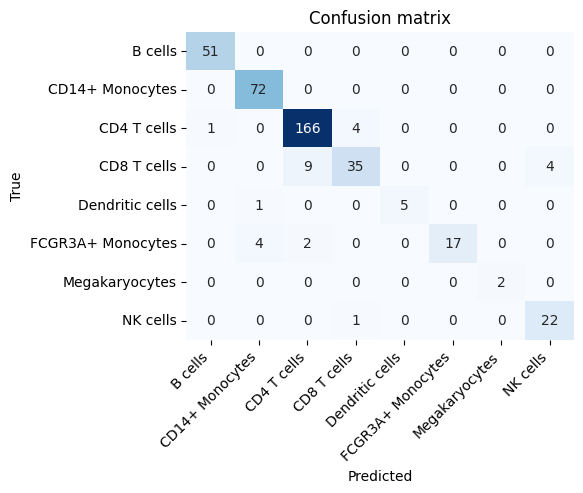
Save a report and inspect the confusion matrix#

The notebook writes its report to artifacts/pbmc_classification/.

runner.save_report(OUTPUT_DIR / "report.md")
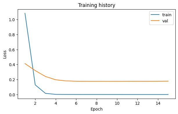
loss_fig, _ = runner.plot_losses()
loss_fig.savefig(OUTPUT_DIR / "loss_curve.png", dpi=150, bbox_inches="tight")
confusion_fig, _ = runner.plot_confusion_matrix()
confusion_fig.savefig(OUTPUT_DIR / "confusion_matrix.png", dpi=150, bbox_inches="tight")
display(confusion_fig)

../_images/81d4625013522671f678fe0bc06bb80cd1c4002cfa9d08a13b337020986c4d88.png

../_images/ee1dff27e884c732df8073a4f8fe3413a2354e60caee85ad2746800c38b83b56.png

Expected outputs#

After running the notebook, check:

accuracy
macro_f1
artifacts/pbmc_classification/report.md
artifacts/pbmc_classification/report.csv
artifacts/pbmc_classification/loss_curve.png
artifacts/pbmc_classification/confusion_matrix.png

Interpretation checklist:

Treat this as a baseline classifier, not a production annotation system.
Read macro F1 before trusting accuracy if the class balance looks uneven.
Use the confusion matrix to see which PBMC groups the model mixes up most often.

If you want a stronger baseline before interpreting the results, switch the first config cell to TUTORIAL_PROFILE = "full" and rerun the notebook.