PBMC model comparison

Audience:

• Researchers who want a quick baseline benchmark before building a custom model.

Prerequisites:

• Install scdlkit[tutorials].

• Know the Scanpy PBMC quickstart notebook first.

Learning goals:

• Compare PCA, autoencoder, vae, and transformer_ae on the same PBMC workflow.

• Inspect the metrics table, runtime, and saved comparison plot.

• Understand whether deep-learning baselines improve on a classical reference.

Install:

python -m pip install "scdlkit[tutorials]"

Outline

1. Load PBMC data with Scanpy.

2. Detect the runtime device.

3. Choose the notebook profile.

4. Run the deep-learning baselines with aligned CPU-friendly settings.

5. Add PCA as a classical reference baseline.

6. Review scalar metrics and runtime.

7. Inspect saved plots and UMAP-style qualitative outputs.

from __future__ import annotations

from pathlib import Path
from time import perf_counter

import numpy as np
import pandas as pd
import scanpy as sc
import torch
from IPython.display import display
from scipy import sparse
from sklearn.decomposition import PCA

from scdlkit import compare_models
from scdlkit.evaluation.metrics import reconstruction_metrics, representation_metrics
from scdlkit.visualization.compare import plot_model_comparison

DATA_PATH = Path("examples/data/pbmc3k_processed.h5ad")
OUTPUT_DIR = Path("artifacts/pbmc_compare")
OUTPUT_DIR.mkdir(parents=True, exist_ok=True)

device_name = "cuda" if torch.cuda.is_available() else "cpu"
print(f"Using device: {device_name}")


def save_umap_from_latent(
    adata,
    latent,
    output_path,
    *,
    label_key="louvain",
    use_rep="X_quality_latent",
):
    plot_adata = adata.copy()
    plot_adata.obsm[use_rep] = latent
    sc.pp.neighbors(plot_adata, use_rep=use_rep)
    sc.tl.umap(plot_adata, random_state=42)
    fig = sc.pl.umap(plot_adata, color=label_key, return_fig=True, frameon=False)
    fig.savefig(output_path, dpi=150, bbox_inches="tight")
    return fig

Using device: cpu

TUTORIAL_PROFILE = "quickstart"  # change to "full" for a longer run

PROFILE = {
    "quickstart": {"epochs": 10, "batch_size": 128},
    "full": {"epochs": 25, "batch_size": 128},
}[TUTORIAL_PROFILE]

TRANSFORMER_MODEL_KWARGS = {
    "patch_size": 48,
    "d_model": 64,
    "n_heads": 2,
    "n_layers": 1,
    "decoder_hidden_dims": (128,),
}

print(f"Tutorial profile: {TUTORIAL_PROFILE}")
print(PROFILE)
print("Compact transformer settings:", TRANSFORMER_MODEL_KWARGS)

Tutorial profile: quickstart
{'epochs': 10, 'batch_size': 128}
Compact transformer settings: {'patch_size': 48, 'd_model': 64, 'n_heads': 2, 'n_layers': 1, 'decoder_hidden_dims': (128,)}

Load PBMC data

The comparison uses the same PBMC dataset as the quickstart tutorial so the main variable is the baseline model, not the preprocessing story.

adata = sc.read_h5ad(DATA_PATH) if DATA_PATH.exists() else sc.datasets.pbmc3k_processed()
print(adata)
print("Label field used for comparison:", "louvain")

AnnData object with n_obs × n_vars = 2638 × 1838
    obs: 'n_genes', 'percent_mito', 'n_counts', 'louvain'
    var: 'n_cells'
    uns: 'draw_graph', 'louvain', 'louvain_colors', 'neighbors', 'pca', 'rank_genes_groups'
    obsm: 'X_pca', 'X_tsne', 'X_umap', 'X_draw_graph_fr'
    varm: 'PCs'
    obsp: 'distances', 'connectivities'
Label field used for comparison: louvain

Compare deep-learning baselines

The benchmark keeps the task, label field, and training settings aligned so the model family is the main variable. The VAE uses a lighter KL term and the Transformer AE uses a compact CPU-friendly configuration so the comparison stays practical in docs and CI. We then add PCA as the classical reference baseline around those deep-learning rows.

from scdlkit import TaskRunner

base_shared_kwargs = {
    "epochs": PROFILE["epochs"],
    "batch_size": PROFILE["batch_size"],
    "label_key": "louvain",
    "device": "auto",
}

ae_result = compare_models(
    adata,
    models=["autoencoder"],
    task="representation",
    shared_kwargs=base_shared_kwargs,
    output_dir=str(OUTPUT_DIR / "autoencoder"),
)

transformer_started_at = perf_counter()
transformer_runner = TaskRunner(
    model="transformer_ae",
    task="representation",
    output_dir=str(OUTPUT_DIR / "transformer_ae"),
    model_kwargs=TRANSFORMER_MODEL_KWARGS,
    **base_shared_kwargs,
)
transformer_runner.fit(adata)
transformer_metrics = transformer_runner.evaluate()
transformer_runtime_sec = perf_counter() - transformer_started_at
transformer_row = pd.DataFrame([
    {
        "model": "transformer_ae",
        "runtime_sec": transformer_runtime_sec,
        **{
            key: value
            for key, value in transformer_metrics.items()
            if isinstance(value, (int, float))
        },
    }
])

vae_started_at = perf_counter()
vae_runner = TaskRunner(
    model="vae",
    task="representation",
    output_dir=str(OUTPUT_DIR / "vae"),
    model_kwargs={"kl_weight": 1e-3},
    **base_shared_kwargs,
)
vae_runner.fit(adata)
vae_metrics = vae_runner.evaluate()
vae_runtime_sec = perf_counter() - vae_started_at
vae_row = pd.DataFrame([
    {
        "model": "vae",
        "runtime_sec": vae_runtime_sec,
        **{
            key: value
            for key, value in vae_metrics.items()
            if isinstance(value, (int, float))
        },
    }
])

deep_metrics = (
    pd.concat([ae_result.metrics_frame, transformer_row, vae_row], ignore_index=True)
    .sort_values("model")
    .reset_index(drop=True)
)
deep_runners = {
    **ae_result.runners,
    "transformer_ae": transformer_runner,
    "vae": vae_runner,
}
deep_metrics

	model	runtime_sec	mse	mae	pearson	spearman	silhouette	knn_label_consistency	ari	nmi
0	autoencoder	3.790278	0.819990	0.402071	0.233890	0.119797	0.164523	0.898990	0.595096	0.768695
1	transformer_ae	7.107681	0.840910	0.407200	0.173332	0.074018	0.048607	0.689394	0.275133	0.397407
2	vae	3.059811	0.820916	0.399915	0.230418	0.115319	0.175449	0.898990	0.588731	0.770850

Add PCA as the classical reference baseline

A baseline-first toolkit should not compare deep-learning models only against each other. Here we add a PCA row with the same representation and reconstruction metrics, then overwrite the saved comparison CSV and plot with the combined view.

x_matrix = adata.X.toarray() if sparse.issparse(adata.X) else np.asarray(adata.X, dtype="float32")
labels = pd.Categorical(adata.obs["louvain"].astype(str)).codes.astype(int)

pca_started_at = perf_counter()
pca = PCA(n_components=min(32, x_matrix.shape[0] - 1, x_matrix.shape[1]), random_state=42)
pca_latent = pca.fit_transform(x_matrix)
pca_reconstruction = pca.inverse_transform(pca_latent)
pca_runtime_sec = perf_counter() - pca_started_at

pca_metrics = reconstruction_metrics(x_matrix, pca_reconstruction)
pca_metrics.update(representation_metrics(pca_latent, labels, None))
pca_row = pd.DataFrame([
    {
        "model": "pca",
        "runtime_sec": pca_runtime_sec,
        **pca_metrics,
    }
])
combined_metrics = (
    pd.concat([pca_row, deep_metrics], ignore_index=True)
    .sort_values("model")
    .reset_index(drop=True)
)
combined_metrics.to_csv(OUTPUT_DIR / "benchmark_metrics.csv", index=False)
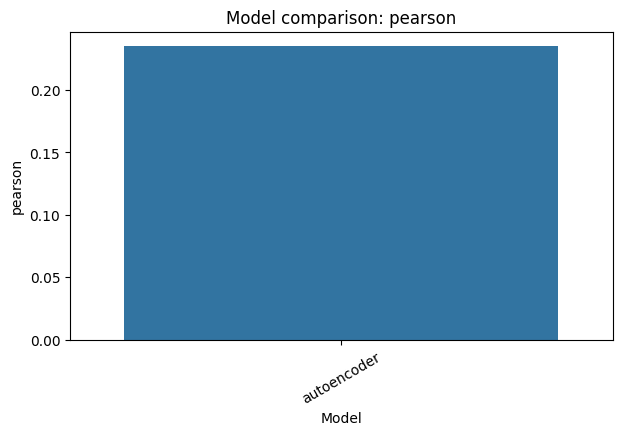
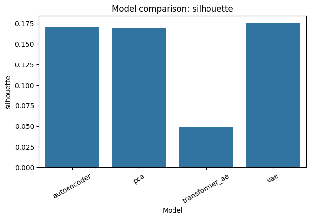
comparison_fig, _ = plot_model_comparison(combined_metrics, metric="silhouette")
comparison_fig.savefig(OUTPUT_DIR / "benchmark_comparison.png", dpi=150, bbox_inches="tight")
display(comparison_fig)
combined_metrics

	model	runtime_sec	mse	mae	pearson	spearman	silhouette	knn_label_consistency	ari	nmi
0	autoencoder	3.790278	0.819990	0.402071	0.233890	0.119797	0.164523	0.898990	0.595096	0.768695
1	pca	0.329488	0.780000	0.416987	0.317878	0.169146	0.170164	0.948067	0.650855	0.798312
2	transformer_ae	7.107681	0.840910	0.407200	0.173332	0.074018	0.048607	0.689394	0.275133	0.397407
3	vae	3.059811	0.820916	0.399915	0.230418	0.115319	0.175449	0.898990	0.588731	0.770850

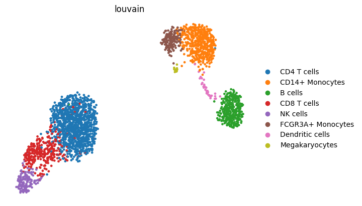
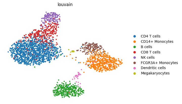
Inspect qualitative outputs

Quantitative metrics should be matched with a qualitative check. Here the notebook saves one UMAP from the PCA reference and one UMAP from the strongest deep-learning baseline by silhouette.

pca_fig = save_umap_from_latent(
    adata,
    pca_latent,
    OUTPUT_DIR / "pca_reference_umap.png",
    use_rep="X_pca_reference",
)
display(pca_fig)

best_deep_row = deep_metrics.sort_values("silhouette", ascending=False).iloc[0]
best_deep_model = best_deep_row["model"]
best_runner = deep_runners[best_deep_model]
best_fig = save_umap_from_latent(
    adata,
    best_runner.encode(adata),
    OUTPUT_DIR / "best_baseline_umap.png",
    use_rep="X_best_baseline",
)
display(best_fig)

Generated outputs and interpretation

The comparison writes its combined outputs to artifacts/pbmc_compare/.

Interpret the table in this order:

1. Check whether the deep-learning baselines beat PCA on the representation metrics.

2. Check how much runtime that gain costs.

3. Use the UMAP-style outputs to make sure the scalar metrics match the qualitative structure.

best_overall = combined_metrics.sort_values("silhouette", ascending=False).iloc[0]
fastest_overall = combined_metrics.sort_values("runtime_sec", ascending=True).iloc[0]
print(f"Best model by silhouette: {best_overall['model']}")
print(f"Fastest model by runtime_sec: {fastest_overall['model']}")

Best model by silhouette: vae
Fastest model by runtime_sec: pca

combined_output_paths = {
    "metrics_csv": str(OUTPUT_DIR / "benchmark_metrics.csv"),
    "comparison_png": str(OUTPUT_DIR / "benchmark_comparison.png"),
    "pca_umap_png": str(OUTPUT_DIR / "pca_reference_umap.png"),
    "best_model_umap_png": str(OUTPUT_DIR / "best_baseline_umap.png"),
}
combined_output_paths

{'metrics_csv': 'artifacts/pbmc_compare/benchmark_metrics.csv',
 'comparison_png': 'artifacts/pbmc_compare/benchmark_comparison.png',
 'pca_umap_png': 'artifacts/pbmc_compare/pca_reference_umap.png',
 'best_model_umap_png': 'artifacts/pbmc_compare/best_baseline_umap.png'}