3. Machine Learning Fundamentals with scikit-learn

Welcome to Module 3! With Python basics and data manipulation tools under our belt, we can now explore the core concepts of Machine Learning (ML). scikit-learn is the cornerstone library for classical ML in Python, offering efficient tools for data analysis and machine learning tasks.

Learning Objectives

After this module, you will be able to:

• Distinguish between Supervised and Unsupervised Learning paradigms.
• Understand the difference between Classification and Regression problems.
• Train basic ML models using scikit-learn’s common API (.fit(), .predict()).
• Evaluate model performance using appropriate metrics (accuracy, confusion matrix, etc.).
• Grasp the concepts of Feature Selection/Engineering.
• Understand the importance of Cross-Validation and Hyperparameter Tuning.

Supervised vs. Unsupervised Learning

Machine learning algorithms are often categorized into two main types based on the kind of data they learn from:

• Supervised Learning:
  • The algorithm learns from a labeled dataset, meaning each data point has both input features and a known output label or target value.
  • Goal: To learn a mapping function that can predict the output for new, unseen input data.
  • Examples: Predicting house prices (output = price), classifying emails as spam/not spam (output = spam/not spam).
• Unsupervised Learning:
  • The algorithm learns from an unlabeled dataset, meaning the data only has input features without corresponding output labels.
  • Goal: To find hidden patterns, structures, or relationships within the data.
  • Examples: Grouping similar customers based on purchasing behavior (clustering), reducing the number of features while preserving information (dimensionality reduction).

Classification and Regression

These are the two main types of Supervised Learning problems:

• Classification:
  • The goal is to predict a discrete category or class label.
  • The output variable is categorical.
  • Examples: Spam detection (spam/not spam), image recognition (cat/dog/bird), sentiment analysis (positive/negative/neutral).
• Regression:
  • The goal is to predict a continuous numerical value.
  • The output variable is numeric.
  • Examples: Predicting temperature, forecasting stock prices, estimating house values.

Scikit-learn Example (Conceptual):

# --- Classification Example ---
from sklearn.linear_model import LogisticRegression # A common classification algorithm
from sklearn.model_selection import train_test_split
import numpy as np

# Assume X represents features (e.g., email word counts), y represents labels (0=not spam, 1=spam)
# We'd typically load real data using Pandas here
X_clf = np.random.rand(100, 5) # Dummy features (100 samples, 5 features)
y_clf = np.random.randint(0, 2, 100) # Dummy labels (0 or 1)

# Split data for training and testing (important!)
X_train_clf, X_test_clf, y_train_clf, y_test_clf = train_test_split(X_clf, y_clf, test_size=0.3, random_state=42)

# Create and train the model
clf_model = LogisticRegression()
clf_model.fit(X_train_clf, y_train_clf) # Learn from training data

# Make predictions on new data
predictions_clf = clf_model.predict(X_test_clf)
print(f"Sample Classification Predictions: {predictions_clf[:10]}") # Show first 10 predictions

# --- Regression Example ---
from sklearn.linear_model import LinearRegression # A common regression algorithm

# Assume X represents features (e.g., house size), y represents the target value (e.g., price)
X_reg = np.random.rand(100, 1) * 1000 # Dummy feature (house size)
y_reg = 50 + 3 * X_reg.flatten() + np.random.randn(100) * 20 # Dummy target (price = 50 + 3*size + noise)

X_train_reg, X_test_reg, y_train_reg, y_test_reg = train_test_split(X_reg, y_reg, test_size=0.3, random_state=42)

# Create and train the model
reg_model = LinearRegression()
reg_model.fit(X_train_reg, y_train_reg) # Learn from training data

# Make predictions on new data
predictions_reg = reg_model.predict(X_test_reg)
print(f"\nSample Regression Predictions: {predictions_reg[:5]}") # Show first 5 predictions

Model Evaluation and Metrics

How do we know if our model is any good? We need to evaluate its performance on data it hasn’t seen during training (the test set). The metrics used depend on whether it’s a classification or regression problem.

Common Classification Metrics:

• Accuracy: The simplest metric; the proportion of correct predictions. (Correct Predictions / Total Predictions). Can be misleading if classes are imbalanced (e.g., 99% not spam, 1% spam).
• Confusion Matrix: A table summarizing prediction results, showing True Positives (TP), True Negatives (TN), False Positives (FP), and False Negatives (FN). Essential for understanding where the model makes mistakes.
• Precision: TP / (TP + FP). Of all the predictions the model made for the positive class, how many were actually positive? Important when the cost of False Positives is high.
• Recall (Sensitivity): TP / (TP + FN). Of all the actual positive instances, how many did the model correctly identify? Important when the cost of False Negatives is high.
• F1-Score: The harmonic mean of Precision and Recall (2 * (Precision * Recall) / (Precision + Recall)). Good measure when you need a balance between Precision and Recall.

Common Regression Metrics:

• Mean Absolute Error (MAE): The average absolute difference between predicted and actual values.
• Mean Squared Error (MSE): The average of the squared differences between predicted and actual values. Penalizes larger errors more heavily.
• Root Mean Squared Error (RMSE): The square root of MSE. Interpretable in the same units as the target variable.
• R-squared (R²): Coefficient of determination. Represents the proportion of the variance in the dependent variable that is predictable from the independent variables. Ranges from 0 to 1 (higher is better).

Scikit-learn Evaluation Example:

# --- Classification Evaluation ---
from sklearn.metrics import accuracy_score, confusion_matrix, classification_report, ConfusionMatrixDisplay
import matplotlib.pyplot as plt

# Using predictions from the classification example above
accuracy = accuracy_score(y_test_clf, predictions_clf)
print(f"\nClassification Accuracy: {accuracy:.4f}")

print("\nClassification Report:")
print(classification_report(y_test_clf, predictions_clf))

# Calculate and display the confusion matrix
cm = confusion_matrix(y_test_clf, predictions_clf)
print("\nConfusion Matrix:\n", cm)

# Visualize the confusion matrix (requires matplotlib)
# Assumes you have run the plot generation script or saved the plot manually
# disp = ConfusionMatrixDisplay(confusion_matrix=cm, display_labels=clf_model.classes_)
# disp.plot()
# plt.title('Confusion Matrix')
# plt.show() # Or savefig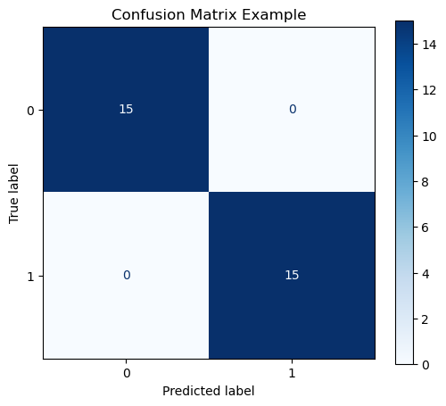

# --- Regression Evaluation ---
from sklearn.metrics import mean_absolute_error, mean_squared_error, r2_score

# Using predictions from the regression example above
mae = mean_absolute_error(y_test_reg, predictions_reg)
mse = mean_squared_error(y_test_reg, predictions_reg)
rmse = np.sqrt(mse) # Or use mean_squared_error(..., squared=False)
r2 = r2_score(y_test_reg, predictions_reg)

print(f"\nRegression MAE: {mae:.2f}")
print(f"Regression MSE: {mse:.2f}")
print(f"Regression RMSE: {rmse:.2f}")
print(f"Regression R-squared: {r2:.4f}")

Feature Selection and Engineering

The quality and relevance of the features (input variables) fed into your model significantly impact its performance.

• Feature Selection: Choosing a subset of the most relevant existing features to use for training. Reduces complexity and can improve performance by removing noise.
• Feature Engineering: Creating new features from existing ones. This might involve:
  • Combining features (e.g., creating an interaction term).
  • Transforming features (e.g., taking logarithms, creating polynomial features).
  • Encoding categorical features into numerical representations (e.g., One-Hot Encoding).
  • Extracting information (e.g., deriving ‘day of week’ from a date).

Cross-Validation and Hyperparameter Tuning

Two crucial techniques for building robust models:

• Cross-Validation (CV): A technique to evaluate how well a model will generalize to an independent dataset. Instead of just one train/test split, the data is split into multiple ‘folds’. The model is trained and evaluated multiple times, using a different fold for testing each time. This gives a more reliable estimate of performance than a single split. K-Fold CV is common.
• Hyperparameter Tuning: Most ML algorithms have ‘hyperparameters’ – settings that are not learned from the data but set before training (e.g., the learning rate, the number of trees in a Random Forest). Finding the optimal hyperparameters is key to good performance. Techniques like Grid Search or Randomized Search systematically try different combinations of hyperparameters, often using cross-validation to evaluate each combination.

Scikit-learn Example (Conceptual):

from sklearn.model_selection import KFold, GridSearchCV
from sklearn.ensemble import RandomForestClassifier # Another classifier

# Assume X, y are your full feature set and labels

# --- Cross-Validation Example ---
kf = KFold(n_splits=5, shuffle=True, random_state=42) # 5-fold CV
scores = []
model_cv = LogisticRegression() # Example model

for fold, (train_index, val_index) in enumerate(kf.split(X_clf)):
    X_train_cv, X_val_cv = X_clf[train_index], X_clf[val_index]
    y_train_cv, y_val_cv = y_clf[train_index], y_clf[val_index]
    
    model_cv.fit(X_train_cv, y_train_cv)
    score = model_cv.score(X_val_cv, y_val_cv) # Uses default metric (accuracy for classifier)
    scores.append(score)
    print(f"Fold {fold+1} Score: {score:.4f}")

print(f"\nAverage CV Score: {np.mean(scores):.4f}")

# --- Hyperparameter Tuning Example (Grid Search) ---
param_grid = {
    'n_estimators': [50, 100, 200], # Number of trees
    'max_depth': [None, 10, 20]     # Max depth of trees
}

# Use a different model for tuning, e.g., RandomForest
rf_model = RandomForestClassifier(random_state=42) 

# GridSearchCV automatically performs cross-validation for each parameter combo
grid_search = GridSearchCV(estimator=rf_model, param_grid=param_grid, cv=3, scoring='accuracy', verbose=1)
# Fit it like a normal model - it will search the grid
# Use the full X_clf, y_clf here usually, as CV handles splitting internally
grid_search.fit(X_clf, y_clf) 

print(f"\nBest Parameters found by Grid Search: {grid_search.best_params_}")
print(f"Best CV Accuracy from Grid Search: {grid_search.best_score_:.4f}")

# The best model found is stored in grid_search.best_estimator_
best_model = grid_search.best_estimator_

Tips & Tricks for Practical ML (incl. Kaggle)

While the fundamentals are crucial, success in applied machine learning and competitions often involves additional strategies:

Practice Exercises (Take-Home Style)

1. Identify Problem Type: For each scenario, state whether it’s primarily Classification or Regression:
   • Predicting the number of stars (1-5) a user will give a movie. (Classification or Regression? Why?)
   • Estimating the total rainfall (in mm) for tomorrow.
   • Determining if a bank transaction is fraudulent (yes/no).
   • Grouping news articles into topics (like ‘sports’, ‘politics’, ’technology’). (Supervised or Unsupervised?)
   • Expected Results: Discussed based on whether the output is categorical or continuous, and whether labels are present. (Movie stars can be argued either way, but often treated as classification/ordinal). Grouping articles is Unsupervised (Clustering).
2. Metrics Interpretation: A classification model achieved 95% accuracy on a dataset where only 5% of instances belong to the positive class. Why might accuracy be a poor metric here? What other metric(s) would be more informative?
   • Expected Result: Accuracy is misleading because a model predicting “negative” for everything would still get 95% accuracy. Precision, Recall, F1-score, or analyzing the Confusion Matrix are better for imbalanced data.
3. Train/Test Split: Use train_test_split from sklearn.model_selection to split a dummy NumPy array X (e.g., 10 rows, 2 columns of random numbers) and a corresponding dummy array y (10 random 0s or 1s) into training and testing sets with a 70/30 split. Print the shapes of X_train, X_test, y_train, y_test.
   • Expected Result: Output should show shapes like X_train: (7, 2), X_test: (3, 2), y_train: (7,), y_test: (3,).
4. Basic Model Training: Import KNeighborsClassifier from sklearn.neighbors. Create an instance, train it on the X_train, y_train data from Exercise 3, and make predictions on X_test. Print the predictions.
   • Expected Result: Output will be an array of 3 predicted labels (0s or 1s), e.g., [0 1 0]. The exact values depend on the random dummy data.

Summary

You’ve learned the fundamental concepts differentiating supervised (classification, regression) and unsupervised learning. You saw the basic scikit-learn API pattern for training and predicting, the importance of evaluating models using appropriate metrics (like accuracy and confusion matrices), and the necessity of techniques like feature engineering, cross-validation, and hyperparameter tuning for building robust and well-performing machine learning models.

Additional Resources

• Scikit-learn User Guide: The essential resource for understanding all scikit-learn functionalities.
• Scikit-learn API Reference: Detailed documentation for specific classes and functions.
• Introduction to Machine Learning with Python by Andreas C. Müller & Sarah Guido: A practical book focusing heavily on scikit-learn.
• StatQuest: Machine Learning Playlist (YouTube): Clear visual explanations of many ML concepts.

Next: Let’s dive deeper into a powerful class of models - Neural Networks! Proceed to Module 4: Introduction to Neural Networks with PyTorch.