2. Data Manipulation with NumPy and Pandas
Welcome to Module 2! Now that you have a foundation in Python basics, we’ll dive into two essential libraries that form the bedrock of data manipulation and analysis in the Python AI ecosystem: NumPy and Pandas. Efficiently handling and preparing data is a critical step in any AI project.
Learning Objectives
After this module, you will be able to:
- Create and manipulate NumPy arrays for efficient numerical computation.
- Understand and perform common array operations and broadcasting.
- Create, index, and manipulate Pandas Series and DataFrames.
- Load data into DataFrames (e.g., from CSV files).
- Perform basic data cleaning tasks like handling missing values.
- Create fundamental data visualizations using Matplotlib and Seaborn.
Foundational Concepts Recap
Before we jump into code, let’s briefly touch upon some mathematical concepts that underpin NumPy, Pandas, and many AI techniques. Don’t worry if you’re not an expert; the goal here is conceptual understanding.
Essential Linear Algebra
Linear algebra deals with vectors, matrices, and their transformations. It’s the language of data representation for many machine learning models.
- Scalars: Single numbers (e.g.,
5,3.14). - Vectors: Ordered lists of numbers, representing points or directions in space (e.g., a data point with multiple features
[1.2, 3.4, 0.9]). NumPy 1D arrays are vectors. - Matrices: Rectangular arrays of numbers, often representing datasets (rows are samples, columns are features) or transformations. NumPy 2D arrays are matrices.
- Key Operations: Operations like vector addition, scalar multiplication, and especially the dot product (fundamental for calculating weighted sums in neural networks) are efficiently handled by NumPy.
Essential Statistics
Statistics helps us describe, analyze, and interpret data. Pandas provides tools built upon these concepts.
- Descriptive Statistics: Ways to summarize data:
- Mean: The average value.
- Median: The middle value when data is sorted.
- Mode: The most frequent value.
- Measures of Spread: How varied the data is:
- Variance / Standard Deviation: Measure how much data points typically deviate from the mean.
- Distributions: How data points are spread out (e.g., the bell curve or Normal Distribution is very common).
- Correlation: Measures the relationship between two variables.
.mean(), .median(), .std()) for your columns. Understanding these helps you explore your data (EDA), identify outliers, and make decisions about data cleaning and feature engineering. Visualizations often aim to reveal statistical properties or distributions.Further Learning Resources
If you want to strengthen your understanding of these foundational topics, consider these resources:
- Linear Algebra:
- Khan Academy - Linear Algebra
- 3Blue1Brown - Essence of Linear Algebra (YouTube Playlist) (Excellent visual intuition)
- Statistics:
- Khan Academy - Statistics and Probability
- StatQuest with Josh Starmer (YouTube Channel) (Clear explanations of stats/ML concepts)
NumPy Arrays and Operations
NumPy (Numerical Python) is the fundamental package for scientific computing in Python. Its core feature is the powerful N-dimensional array object (ndarray). NumPy arrays are more efficient for numerical operations than standard Python lists, especially for large datasets.
Creating Arrays:
import numpy as np # Standard alias for NumPy

# Create from a Python list
list_data = [1, 2, 3, 4, 5]
np_array = np.array(list_data)
print(f"NumPy array: {np_array}")
print(f"Array type: {np_array.dtype}") # Check data type

# Create arrays with specific values
zeros_array = np.zeros((2, 3)) # 2x3 array of zeros (shape specified as a tuple)
print("\nZeros array:\n", zeros_array)

ones_array = np.ones(4) # 1D array of ones
print("\nOnes array:", ones_array)

# Create sequences
range_array = np.arange(0, 10, 2) # Like Python's range, but creates an array (start, stop, step)
print("\nRange array:", range_array)
Array Operations (Element-wise):
Most standard math operations work element-wise on NumPy arrays.
a = np.array([1, 2, 3])
b = np.array([4, 5, 6])

# Element-wise addition, subtraction, multiplication
print(f"a + b = {a + b}")
print(f"a * b = {a * b}")

# Operations with scalars
print(f"a * 2 = {a * 2}")
print(f"a ** 2 = {a ** 2}") # Squaring each element

# Universal functions (ufuncs)
print(f"Square root of a: {np.sqrt(a)}")
Broadcasting: NumPy can often perform operations between arrays of different shapes if certain rules are met (this is called broadcasting).
matrix = np.array([[1, 2, 3], [4, 5, 6]]) # 2x3 matrix
vector = np.array([10, 20, 30])        # 1x3 vector

# Add the vector to each row of the matrix
result = matrix + vector
print("\nMatrix + Vector (Broadcasting):\n", result)Pandas DataFrames and Series
Pandas builds on NumPy and provides high-performance, easy-to-use data structures and data analysis tools. The two primary data structures are:
Series: A one-dimensional labeled array (like a column in a spreadsheet).DataFrame: A two-dimensional labeled data structure with columns of potentially different types (like a whole spreadsheet or SQL table). This is the most commonly used Pandas object.
Creating Series and DataFrames:
import pandas as pd # Standard alias for Pandas

# Creating a Series
s = pd.Series([0.1, 0.2, 0.3, 0.4], index=['a', 'b', 'c', 'd'])
print("Pandas Series:\n", s)

# Creating a DataFrame from a dictionary
data = {
    'FeatureA': [1.0, 2.5, 3.1, 4.7],
    'FeatureB': ['cat', 'dog', 'cat', 'rabbit'],
    'Target': [0, 1, 0, 1]
}
df = pd.DataFrame(data)
print("\nPandas DataFrame:\n", df)
Data Loading (e.g., CSV): Pandas excels at reading data from various file formats.
# Assuming you have a CSV file named 'data.csv'
# Example CSV content:
# ID,Temperature,Humidity
# 1,25.5,60
# 2,26.1,62
# 3,24.9,58

# Use a try-except block for robust file reading
try:
    # Create a dummy CSV for the example
    with open('data.csv', 'w') as f:
        f.write("ID,Temperature,Humidity\n")
        f.write("1,25.5,60\n")
        f.write("2,26.1,62\n")
        f.write("3,24.9,58\n")
        f.write("4,,55\n") # Add a row with missing temperature

    df_from_csv = pd.read_csv('data.csv')
    print("\nDataFrame loaded from CSV:\n", df_from_csv)

except FileNotFoundError:
    print("\nError: data.csv not found. Create the file to run this example.")
except Exception as e:
    print(f"\nAn error occurred reading CSV: {e}")
Selection and Indexing: Accessing data within a DataFrame is crucial.
# Select a single column (returns a Series)
temperatures = df_from_csv['Temperature']
print("\nTemperatures Series:\n", temperatures)

# Select multiple columns (returns a DataFrame)
subset_df = df_from_csv[['ID', 'Humidity']]
print("\nSubset DataFrame:\n", subset_df)

# Select rows based on index (.loc) or integer position (.iloc)
print("\nRow with index 1 (.loc):\n", df_from_csv.loc[1])
print("\nFirst row (.iloc):\n", df_from_csv.iloc[0])

# Conditional selection (Boolean indexing)
high_humidity_df = df_from_csv[df_from_csv['Humidity'] > 60]
print("\nRows with Humidity > 60:\n", high_humidity_df)Data Cleaning and Preprocessing
Real-world data is rarely perfect. Data cleaning involves handling issues like missing values, incorrect data types, or outliers.
Handling Missing Values (NaN): Pandas represents missing values typically as NaN (Not a Number).
print("\nDataFrame with potential missing values:\n", df_from_csv)

# Check for missing values
print("\nMissing values per column:\n", df_from_csv.isnull().sum())

# Option 1: Drop rows with any missing values
df_dropped = df_from_csv.dropna()
print("\nDataFrame after dropping NaN rows:\n", df_dropped)

# Option 2: Fill missing values (e.g., with the mean)
mean_temp = df_from_csv['Temperature'].mean()
df_filled = df_from_csv.fillna({'Temperature': mean_temp}) # Fill specific column
print("\nDataFrame after filling NaN temperature with mean:\n", df_filled)Data Visualization with Matplotlib and Seaborn
Visualizing data is essential for understanding patterns, trends, and relationships before and after modeling.
- Matplotlib: The foundational plotting library in Python. Provides fine-grained control.
- Seaborn: Built on top of Matplotlib, offers higher-level functions for creating informative and attractive statistical graphics.
import matplotlib.pyplot as plt # Standard alias
import seaborn as sns          # Standard alias

# Ensure plots show up in Jupyter environments
# %matplotlib inline  # Uncomment this line if using Jupyter Notebook/Lab

# Use the DataFrame with filled values for plotting
df_plot = df_filled

# --- Simple Matplotlib Plot ---
plt.figure(figsize=(8, 4)) # Create a figure and set its size
plt.plot(df_plot['ID'], df_plot['Temperature'], marker='o', linestyle='-')
plt.title('Temperature Trend')
plt.xlabel('ID')
plt.ylabel('Temperature (°C)')
plt.grid(True)
# plt.savefig('static/images/numpy-pandas/temp_trend.png') # Example save command
plt.show() # Display the plot (or save it)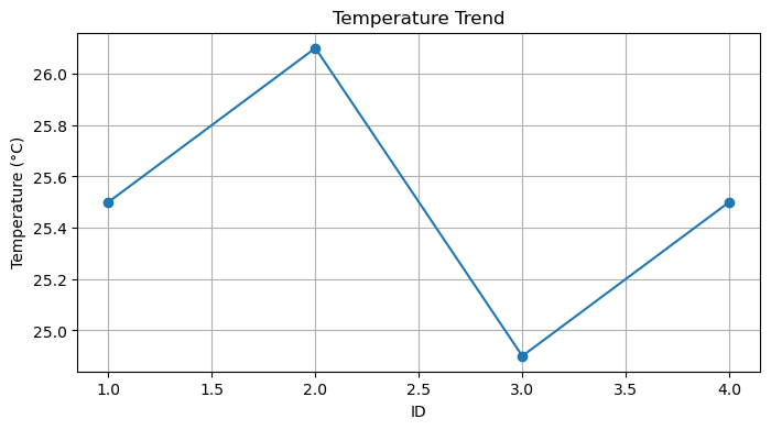
# --- Seaborn Plots ---

# Histogram of Humidity
plt.figure(figsize=(8, 4))
sns.histplot(data=df_plot, x='Humidity', kde=True) # kde adds a density curve
plt.title('Humidity Distribution')
# plt.savefig('static/images/numpy-pandas/humidity_hist.png')
plt.show()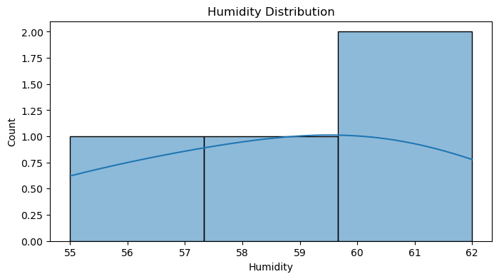
# Scatter plot to see relationship between Temperature and Humidity
plt.figure(figsize=(8, 4))
sns.scatterplot(data=df_plot, x='Temperature', y='Humidity')
plt.title('Temperature vs. Humidity')
# plt.savefig('static/images/numpy-pandas/temp_vs_humidity_scatter.png')
plt.show()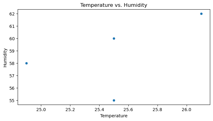
# Box plot (useful for comparing distributions or finding outliers)
# Let's add a dummy category for demonstration
# Assuming df_plot exists and we add the Category column
df_plot['Category'] = ['A', 'A', 'B', 'B']
plt.figure(figsize=(8, 4))
sns.boxplot(data=df_plot, x='Category', y='Temperature')
plt.title('Temperature Distribution by Category')
# plt.savefig('static/images/numpy-pandas/temp_by_cat_boxplot.png')
plt.show()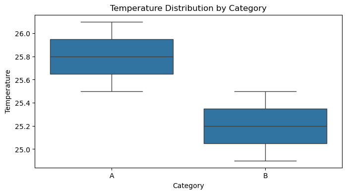
AI Relevance: Exploratory Data Analysis (EDA) relies heavily on visualization. You’ll use plots to:
- Understand feature distributions (histograms).
- Identify relationships between features (scatter plots).
- Compare groups (box plots).
- Visualize model predictions vs. actual values.
- Diagnose model performance (e.g., plotting loss curves during training).
Practice Exercises (Take-Home Style)
- NumPy Array Creation: Create a 3x3 NumPy array containing numbers from 1 to 9. Then, multiply every element in the array by 10.
- Expected Result:
[[ 10,  20,  30],
 [ 40,  50,  60],
 [ 70,  80,  90]]
- Expected Result:
- Pandas DataFrame: Create a Pandas DataFrame with two columns, ‘Student’ (containing names: ‘Alice’, ‘Bob’, ‘Charlie’) and ‘Score’ (containing scores: 85, 92, 78). Select and print only the ‘Score’ column.
- Expected Result: A Pandas Series containing the scores:
0    85
1    92
2    78
Name: Score, dtype: int64
- Expected Result: A Pandas Series containing the scores:
- Conditional Selection: Using the DataFrame from Exercise 2, select and print the rows where the ‘Score’ is greater than 90.
- Expected Result: A DataFrame containing Bob’s row:
   Student  Score
1     Bob     92
- Expected Result: A DataFrame containing Bob’s row:
- Missing Value Handling: Create a DataFrame with a column containing
[10, 20, np.nan, 40]. Calculate the mean of the column (ignoring NaN) and then fill the missing value with this mean. Print the final DataFrame.- Expected Result: The NaN should be replaced by 23.33… (the mean of 10, 20, 40). The DataFrame should look similar to:
      0
0  10.000000
1  20.000000
2  23.333333
3  40.000000
- Expected Result: The NaN should be replaced by 23.33… (the mean of 10, 20, 40). The DataFrame should look similar to:
- Simple Plot: Using the DataFrame from Exercise 2, create a simple bar chart showing the scores for each student using Matplotlib or Seaborn.
- Expected Result: A bar chart displaying three bars for Alice, Bob, and Charlie with heights corresponding to their scores.
Summary
NumPy provides the foundation for numerical computing with its efficient arrays, while Pandas offers powerful and flexible DataFrames for handling structured data. Matplotlib and Seaborn are essential for visualizing your data to gain insights. Mastering these libraries is crucial for nearly all data preprocessing, exploration, and feature engineering tasks in AI.
Additional Resources
- NumPy Documentation: The official source for all things NumPy.
- Pandas Documentation: Comprehensive guides and API reference.
- Matplotlib Documentation: Explore the vast capabilities of Matplotlib.
- Seaborn Documentation: Tutorials and examples for statistical visualization.
- Python Data Science Handbook by Jake VanderPlas: An excellent online book covering NumPy, Pandas, Matplotlib, and more.
Next: Ready to build predictive models? Proceed to Module 3: Machine Learning Fundamentals with scikit-learn.