6. Computer Vision Essentials

Welcome to Module 6! We now delve into Computer Vision (CV), a field of AI focused on how computers can gain high-level understanding from digital images or videos. From self-driving cars recognizing pedestrians to medical image analysis, CV has widespread applications. This module introduces core concepts and popular libraries like OpenCV, building upon the neural network foundations from Module 4.

Learning Objectives

After this module, you will be able to:

• Perform basic image loading, manipulation, and display using OpenCV.
• Understand common image processing techniques like color space conversion, filtering, and edge detection.
• Explain how Convolutional Neural Networks (CNNs) are applied to image classification.
• Describe the task of Object Detection and common approaches.
• Understand the basic concepts behind Face Recognition.
• Grasp the goal of Image Segmentation.

Image Processing with OpenCV

OpenCV (Open Source Computer Vision Library) is the workhorse library for many computer vision tasks. It provides a vast array of functions for reading, writing, manipulating, and analyzing images and videos.

Basic Operations:

• Reading Images: Loading an image from a file. OpenCV typically loads images in BGR (Blue, Green, Red) format by default, unlike Matplotlib which expects RGB.
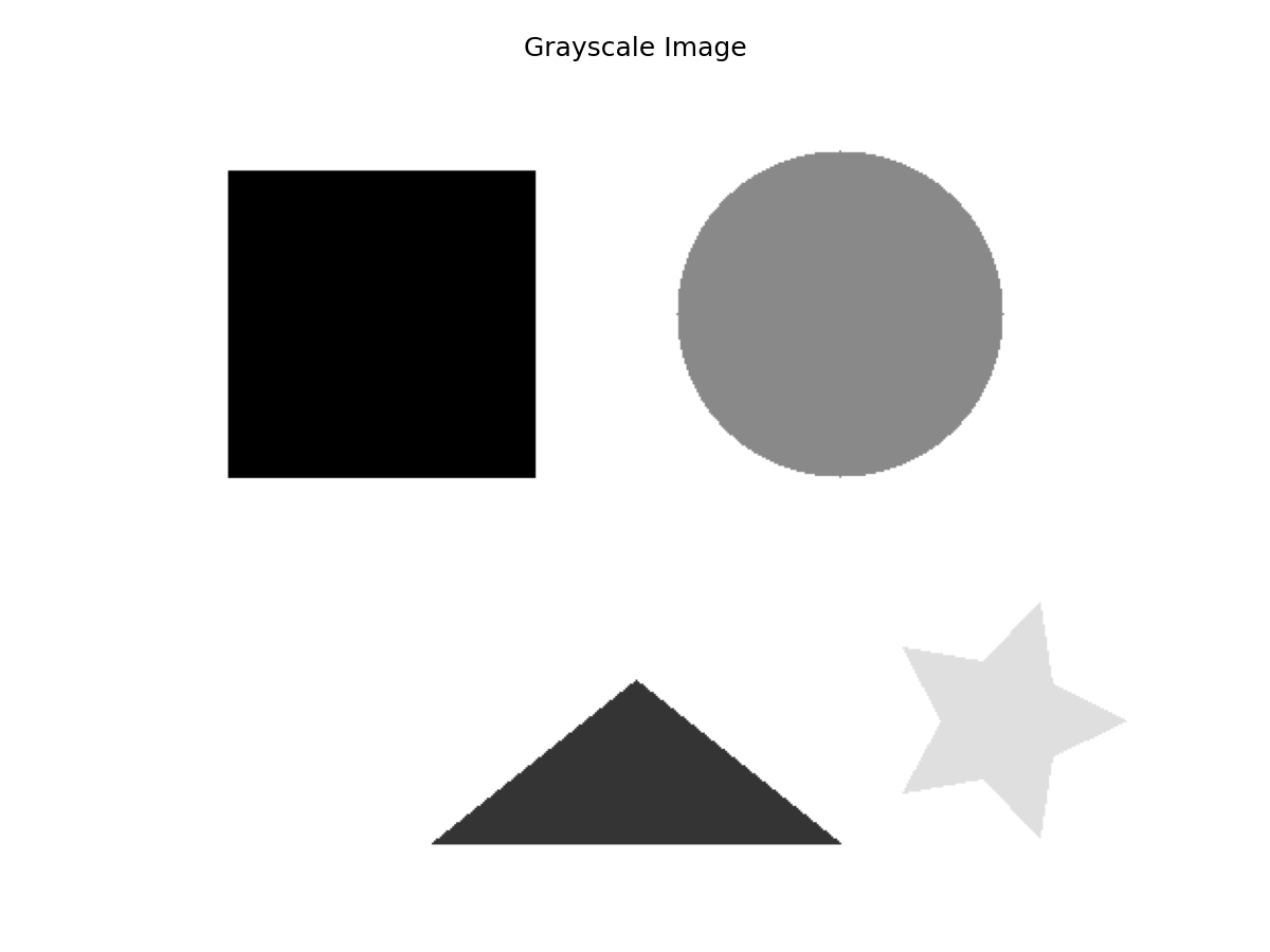
• Color Spaces: Converting between color spaces (e.g., BGR to Grayscale, BGR to RGB, BGR to HSV). Grayscale is often used to simplify processing.
• Resizing: Changing the dimensions of an image.
• Filtering/Blurring: Applying filters (kernels) to smooth images, reduce noise, or sharpen details (e.g., Gaussian Blur, Median Blur).
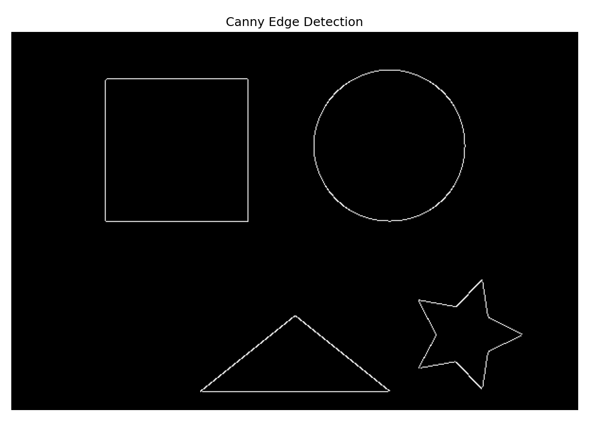
• Edge Detection: Identifying sharp changes in intensity, often corresponding to object boundaries (e.g., Canny Edge Detector).

OpenCV Example:

import cv2 # OpenCV library
import matplotlib.pyplot as plt
import numpy as np # Often used with OpenCV

# --- Reading and Displaying an Image ---
# Make sure you have an image file (e.g., 'test_image.jpg') 
# in the same directory or provide the correct path.
# For this example, let's create a simple dummy image if one doesn't exist
dummy_image_path = 'test_image.jpg'
try:
    img_bgr = cv2.imread(dummy_image_path)
    if img_bgr is None: # Handle file not found or invalid image
        print(f"Warning: '{dummy_image_path}' not found or invalid. Creating a dummy image.")
        img_bgr = np.zeros((100, 150, 3), dtype=np.uint8) # Black image
        img_bgr[30:70, 50:100] = [0, 255, 0] # Add a green rectangle
        cv2.imwrite(dummy_image_path, img_bgr) # Save dummy image
        img_bgr = cv2.imread(dummy_image_path) # Reload it

    print(f"Image shape (Height, Width, Channels): {img_bgr.shape}")

    # Convert BGR (OpenCV default) to RGB for Matplotlib display
    img_rgb = cv2.cvtColor(img_bgr, cv2.COLOR_BGR2RGB)

    plt.figure(figsize=(5,5))
    plt.imshow(img_rgb)
    plt.title('Original Image (RGB)')
    plt.axis('off') # Hide axes
    plt.show()

    # --- Color Space Conversion ---
    img_gray = cv2.cvtColor(img_bgr, cv2.COLOR_BGR2GRAY)
    plt.figure(figsize=(5,5))
    plt.imshow(img_gray, cmap='gray') # Use grayscale colormap
    plt.title('Grayscale Image')
    plt.axis('off')
    plt.show()

    # --- Blurring (Gaussian) ---
    img_blur = cv2.GaussianBlur(img_rgb, (15, 15), 0) # Kernel size (odd numbers), sigma
    plt.figure(figsize=(5,5))
    plt.imshow(img_blur)
    plt.title('Blurred Image')
    plt.axis('off')
    plt.show()

    # --- Edge Detection (Canny) ---
    # Often applied to grayscale images
    edges = cv2.Canny(img_gray, threshold1=100, threshold2=200) # Threshold values
    plt.figure(figsize=(5,5))
    plt.imshow(edges, cmap='gray')
    plt.title('Canny Edges')
    plt.axis('off')
    plt.show()

except Exception as e:
    print(f"An error occurred during OpenCV operations: {e}")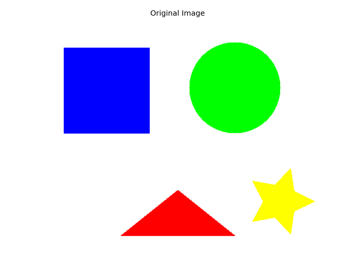

(These images need to be generated/obtained and placed in static/images/cv/)

Image Classification with CNNs

As introduced in Module 4, Convolutional Neural Networks (CNNs) are the dominant approach for image classification.

• Goal: Assign a single label (class) to an entire image (e.g., “cat”, “dog”, “car”).
• How CNNs Work (Recap):
  • Convolutional layers learn spatial hierarchies of features (edges -> textures -> parts -> objects).
  • Pooling layers provide spatial invariance and reduce dimensionality.
  • Fully connected layers at the end perform the final classification based on the learned high-level features.
• Training: Requires a large dataset of labeled images (e.g., ImageNet, CIFAR-10). The network learns to associate visual patterns with specific class labels through backpropagation and gradient descent.
• Transfer Learning: A very common and effective technique where you take a CNN pre-trained on a large dataset (like ImageNet) and fine-tune it on your specific, smaller dataset. This leverages the general features learned by the pre-trained model and significantly reduces the amount of data and training time required.

# Conceptual PyTorch CNN usage (building on Module 4)
import torch
import torch.nn as nn
import torchvision.models as models # Access pre-trained models
import torchvision.transforms as transforms # For image preprocessing
from PIL import Image # Python Imaging Library

# --- Load a pre-trained model (e.g., ResNet18) ---
model_clf = models.resnet18(pretrained=True) 
# Modify the final layer for your specific number of classes
# num_your_classes = ... # Define the number of classes for your specific problem
num_ftrs = model_clf.fc.in_features
model_clf.fc = nn.Linear(num_ftrs, num_your_classes) # Replace final layer

# --- Image Preprocessing ---
# Define transformations required by the pre-trained model
preprocess = transforms.Compose([
    transforms.Resize(256),
    transforms.CenterCrop(224),
    transforms.ToTensor(),
    transforms.Normalize(mean=[0.485, 0.456, 0.406], std=[0.229, 0.224, 0.225]),
])

# --- Load and process an image ---
# image_path = "path/to/your/image.jpg" # Define the path to your image
try:
    img_pil = Image.open(image_path).convert('RGB') # Load as PIL image
    input_tensor = preprocess(img_pil)
    input_batch = input_tensor.unsqueeze(0) # Create a mini-batch as expected by models
except FileNotFoundError:
    print(f"Image file not found at: {image_path}")
    input_batch = None # Handle the case where the image isn't found
except NameError:
    print("Variable 'image_path' is not defined.")
    input_batch = None
except Exception as e:
    print(f"An error occurred loading the image: {e}")
    input_batch = None

# --- Make Prediction ---
if input_batch is not None:
    model_clf.eval() # Set model to evaluation mode
    with torch.no_grad():
        output = model_clf(input_batch)
        # Process output (e.g., apply softmax, get highest probability class)
        probabilities = torch.nn.functional.softmax(output[0], dim=0)
        predicted_class_index = probabilities.argmax().item()
        # Map index to class name based on your dataset labels
        # class_names = [...] # Define your list of class names
        # predicted_class_name = class_names[predicted_class_index] 
        print(f"Predicted Class Index: {predicted_class_index}") 
        # print(f"Predicted Class Name: {predicted_class_name}") 
else:
    print("Skipping prediction due to image loading error.")

Object Detection Basics

Goes beyond classification by identifying multiple objects within an image and locating them with bounding boxes.

• Goal: Predict both the class label (e.g., “car”, “person”) and the coordinates of a bounding box surrounding each object instance.
• Challenges: Handling objects of varying sizes, multiple overlapping objects, different viewpoints, and lighting conditions.
• Common Approaches:
  • Two-Stage Detectors (e.g., R-CNN family: Fast R-CNN, Faster R-CNN): First propose regions likely to contain objects, then classify objects within those regions. Generally accurate but can be slower.
  • One-Stage Detectors (e.g., YOLO - You Only Look Once, SSD - Single Shot MultiBox Detector): Predict bounding boxes and class probabilities directly from the full image in a single pass. Typically faster, making them suitable for real-time applications, potentially with a slight trade-off in accuracy for small objects.

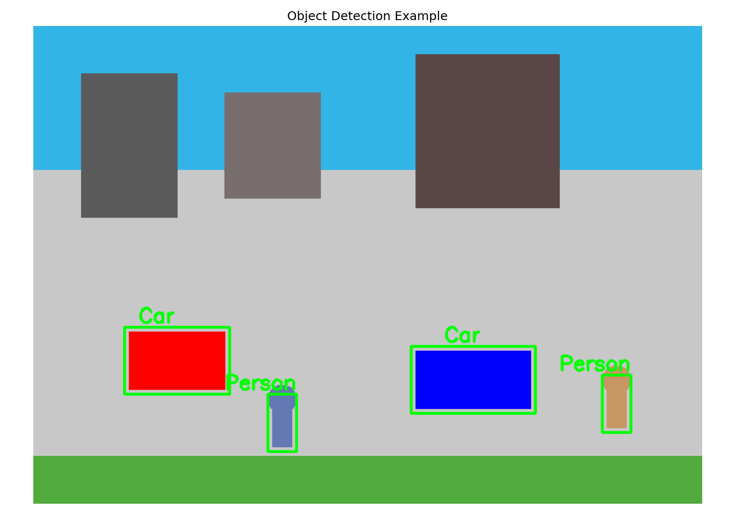(Placeholder for an image showing bounding boxes around objects)

Face Recognition Introduction

A specialized task focusing on identifying or verifying individuals based on their facial features.

• Goal: Match a detected face to a known identity in a database (Recognition/Identification) or verify if two face images belong to the same person (Verification).
• Typical Pipeline:
  1. Face Detection: First, locate faces in the image (using methods like Haar Cascades, HOG, or deep learning detectors).
  2. Face Alignment: Normalize the face pose (e.g., rotate so eyes are level).
  3. Feature Extraction: Extract a numerical feature vector (embedding) that uniquely represents the face’s characteristics. Deep learning models (like FaceNet, ArcFace) are state-of-the-art here.
  4. Matching: Compare the extracted feature vector against vectors of known individuals in a database using distance metrics (e.g., Euclidean distance, cosine similarity).

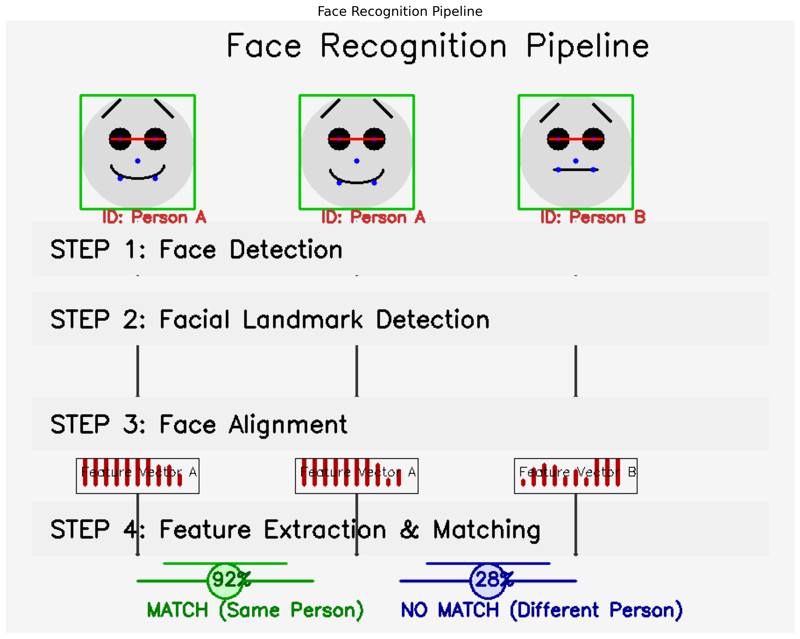A visual representation of the typical face recognition pipeline: detection, alignment, feature extraction, and matching.

Image Segmentation Concepts

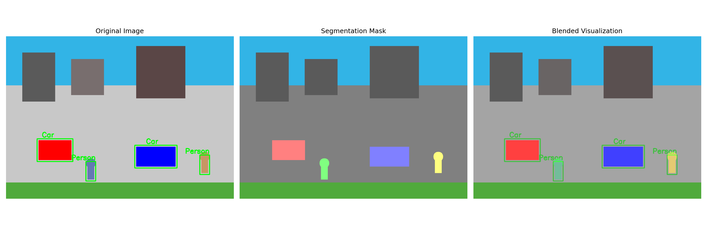
Assigns a class label to every pixel in an image, essentially partitioning the image into meaningful segments.

• Goal: Create a pixel-level mask indicating the exact location and shape of objects.
• Types:
  • Semantic Segmentation: Assigns each pixel to a category (e.g., all pixels belonging to ‘car’, ‘road’, ‘sky’, ‘person’) but doesn’t distinguish between different instances of the same category.
  • Instance Segmentation: Goes further by identifying individual object instances within each category (e.g., labeling ‘person 1’, ‘person 2’, ‘car 1’).
• Applications: Medical imaging (segmenting tumors or organs), autonomous driving (identifying drivable areas, pedestrians), satellite imagery analysis.
• Approaches: Primarily uses deep learning architectures, often based on CNNs with modifications like Fully Convolutional Networks (FCNs) or U-Net architectures.

(Placeholder for an image showing pixel-level masks)

Practice Exercises (Take-Home Style)

1. OpenCV Loading: Write Python code using OpenCV (cv2) to load an image file named my_image.jpg. Convert it to grayscale and display both the original (in RGB) and grayscale versions using Matplotlib. (Handle potential file not found errors).
   • Expected Result: Two plot windows (or inline plots in Jupyter) showing the original color image and its grayscale conversion.
2. CNN Application: What is the primary advantage of using a CNN over a basic feedforward neural network (MLP) for an image classification task?
   • Expected Result: CNNs leverage convolutional layers to effectively learn spatial hierarchies of features and are parameter-efficient due to weight sharing in the filters, making them better suited for the spatial structure of images compared to MLPs which treat pixels independently.
3. CV Task Identification: Match the description to the most appropriate Computer Vision task (Image Classification, Object Detection, Image Segmentation):
   • Drawing boxes around all cats and dogs in a photo.
   • Labeling every pixel in an image as either ‘road’ or ’not road’.
   • Deciding if an X-ray image shows pneumonia or not.
   • Expected Result: Object Detection, Image Segmentation, Image Classification.
4. Transfer Learning: Briefly explain the concept of Transfer Learning in the context of image classification with CNNs. Why is it useful?
   • Expected Result: Using a CNN model pre-trained on a large dataset (like ImageNet) as a starting point for a new task on a smaller dataset. It’s useful because the pre-trained model has already learned general visual features, reducing the need for vast amounts of labeled data and training time for the new task.

Summary

You’ve explored the fundamentals of Computer Vision, starting with basic image processing using OpenCV (loading, color spaces, filtering, edge detection). We revisited CNNs for image classification and discussed the concepts behind more advanced tasks like Object Detection, Face Recognition, and Image Segmentation. These tasks often rely on sophisticated deep learning models.

Additional Resources

• OpenCV Tutorials: Official OpenCV documentation and tutorials.
• PyImageSearch Blog: Many practical tutorials on OpenCV and computer vision.
• CS231n: Convolutional Neural Networks for Visual Recognition (Stanford Course): In-depth university course materials on deep learning for CV.
• Learn OpenCV Blog: Tutorials on various CV and deep learning topics.
• Roboflow Blog: Focuses on practical aspects of dataset creation and model deployment for CV.

Next: Let’s bring many of these concepts together by looking at a practical project implementation in Module 7: Practical AI Project Implementations.